DML ATE Example

This notebook covers scenario:

Is RCT	Treatment	Outcome	EDA	Estimands	Refutation
Observational	Binary	Continuous	Yes	ATE	Yes

We will estimate Average Treatment Effect (ATE) of binary treatment on continuous outcome. It shows explonatary data analysis and refutation tests

Generate data

Let’s generate data of how feature (Treatment) impact on ARPU (Outcome) with linear effect (theta) = 1.8

import numpy as np
import pandas as pd
import matplotlib.pyplot as plt
from causalkit.data import CausalDatasetGenerator, CausalData

# Reproducibility
np.random.seed(42)

confounder_specs = [
    {"name": "tenure_months", "dist": "normal", "mu": 24, "sd": 12},
    {"name": "avg_sessions_week", "dist": "normal", "mu": 5, "sd": 2},
    {"name": "spend_last_month", "dist": "uniform", "a": 0, "b": 200},
    {"name": "premium_user", "dist": "bernoulli", "p": 0.25},
    {"name": "urban_resident", "dist": "bernoulli", "p": 0.60},
]

# Causal effect and noise
theta = 1.8  # ATE: +1.8 ARPU units if new_feature = 1
sigma_y = 3.5  # ARPU noise std
target_t_rate = 0.35  # ~35% treated

# Effects of confounders on ARPU (baseline, additive)
# Order: tenure_months, avg_sessions_week, spend_last_month, premium_user, urban_resident
beta_y = np.array([
    0.05,  # tenure_months: small positive effect
    0.40,  # avg_sessions_week: strong positive effect
    0.02,  # spend_last_month: recent spend correlates with ARPU
    2.00,  # premium_user: premium users have higher ARPU
    1.00,  # urban_resident: urban users slightly higher ARPU
], dtype=float)

# Effects of confounders on treatment assignment (log-odds scale)
beta_t = np.array([
    0.015,  # tenure_months
    0.10,  # avg_sessions_week
    0.002,  # spend_last_month
    0.75,  # premium_user
    0.30,  # urban_resident: more likely to get the feature
], dtype=float)

gen = CausalDatasetGenerator(
    theta=theta,
    outcome_type="continuous",
    sigma_y=sigma_y,
    target_t_rate=target_t_rate,
    seed=42,
    confounder_specs=confounder_specs,
    beta_y=beta_y,
    beta_t=beta_t,
)


# Create dataset
causal_data = gen.to_causal_data(
    n=10000,
    confounders = [
    "tenure_months",
    "avg_sessions_week",
    "spend_last_month",
    "premium_user",
    "urban_resident",
]
)

# Show first few rows
causal_data.df.head()

	y	t	tenure_months	avg_sessions_week	spend_last_month	premium_user	urban_resident
0	5.927714	1.0	27.656605	5.352554	72.552568	1.0	0.0
1	11.122008	1.0	11.520191	6.798247	188.481287	1.0	0.0
2	10.580393	1.0	33.005414	2.055459	51.040440	0.0	1.0
3	6.982844	1.0	35.286777	4.429404	166.992239	0.0	1.0
4	10.899381	0.0	0.587578	6.658307	179.371126	0.0	0.0

EDA

from causalkit.eda import CausalEDA
eda = CausalEDA(causal_data)

---------------------------------------------------------------------------
ModuleNotFoundError                       Traceback (most recent call last)
Cell In[2], line 1
----> 1 from causalkit.eda import CausalEDA
      2 eda = CausalEDA(causal_data)

File ~/work/CausalKit/CausalKit/causalkit/eda/__init__.py:1
----> 1 from .eda import CausalEDA, CausalDataLite
      3 __all__ = ["CausalEDA", "CausalDataLite"]

File ~/work/CausalKit/CausalKit/causalkit/eda/eda.py:37
     35 from sklearn.compose import ColumnTransformer
     36 from sklearn.pipeline import Pipeline
---> 37 from catboost import CatBoostClassifier, CatBoostRegressor
     38 import matplotlib.pyplot as plt
     41 class PropensityModel:

ModuleNotFoundError: No module named 'catboost'

General dataset information

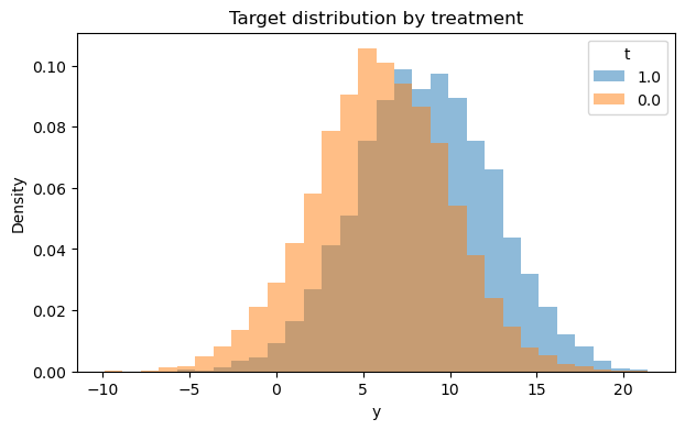
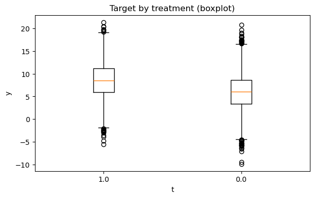
Let’s see how outcome differ between clients who recieved the feature and didn’t

# shape of data
eda.data_shape()

{'n_rows': 10000, 'n_columns': 7}

# 1) Outcome statistics by treatment
eda.outcome_stats()

	count	mean	std	min	p10	p25	median	p75	p90	max
treatment
0.0	6519	6.011340	3.925893	-9.866447	1.012888	3.426894	6.030504	8.676781	10.952265	20.770359
1.0	3481	8.553615	3.934260	-5.507710	3.525225	5.909860	8.566860	11.216054	13.602967	21.377687

# 2) Outcome distribution by treatment (hist + boxplot)
fig1, fig2 = eda.outcome_plots()
plt.show()

Propensity

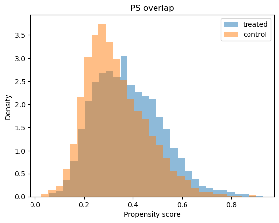
Now let’s examine how propensity score differ treatments

# Shows means of confounders for control/treated groups, absolute differences, and SMD values
confounders_balance_df = eda.confounders_means()
display(confounders_balance_df)

	mean_t_0	mean_t_1	abs_diff	smd
confounders
premium_user	0.198343	0.347889	0.149545	0.340423
avg_sessions_week	4.905841	5.293265	0.387423	0.193959
tenure_months	23.170108	25.200827	2.030718	0.168676
urban_resident	0.578003	0.643781	0.065778	0.135209
spend_last_month	97.801230	105.271930	7.470700	0.129267

# Propensity model fit
ps_model = eda.fit_propensity()

# ROC AUC - shows how predictable treatment is from confounders
roc_auc_score = ps_model.roc_auc
print("ROC AUC from PropensityModel:", round(roc_auc_score, 4))

ROC AUC from PropensityModel: 0.6053

# Positivity check - assess overlap between treatment groups
positivity_result = ps_model.positivity_check()
print("Positivity check from PropensityModel:", positivity_result)

Positivity check from PropensityModel: {'bounds': (0.05, 0.95), 'share_below': 0.0008, 'share_above': 0.0, 'flag': False}

# SHAP values - feature importance for treatment assignment from confounders
shap_values_df = ps_model.shap
display(shap_values_df)

	feature	shap_mean
0	spend_last_month	-0.000322
1	tenure_months	0.000140
2	avg_sessions_week	0.000122
3	premium_user	0.000052
4	urban_resident	0.000008

# Propensity score overlap graph
ps_model.ps_graph()
plt.show()

Outcome regression

Let’s analyze how confounders predict outcome

# Outcome model fit
outcome_model = eda.outcome_fit()

# RMSE and MAE of regression model
print(outcome_model.scores)

{'rmse': 3.6896558290948964, 'mae': 2.94099663606919}

# 2) SHAP values - feature importance for outcome prediction from confounders
shap_outcome_df = outcome_model.shap
display(shap_outcome_df)

	feature	shap_mean
0	spend_last_month	0.002252
1	tenure_months	-0.001747
2	avg_sessions_week	-0.000951
3	premium_user	0.000729
4	urban_resident	-0.000282

Inference

Now time to estimate ATE with Double Machine Learning

from causalkit.inference.ate import dml_ate

# Estimate Average Treatment Effect (ATE)
ate_result = dml_ate(causal_data, n_folds=3, confidence_level=0.95)

ate_result

{'coefficient': 1.7547754158492368,
 'std_error': 0.08120639822820347,
 'p_value': 1.4835396169728733e-103,
 'confidence_interval': (1.5956138000077407, 1.913937031690733),
 'model': <doubleml.irm.irm.DoubleMLIRM at 0x157b9fed0>}

True theta in our data generating proccess was 1.8

Refutation

Placebo

# Import refutation utilities
from causalkit.refutation import (
    refute_placebo_outcome,
    refute_placebo_treatment,
    refute_subset,
    refute_irm_orthogonality,
    sensitivity_analysis,
    sensitivity_analysis_set
)

Replacing outcome with dummy random variable must broke our model and effect will be near zero

# Replacing an outcome with placebo
ate_placebo_outcome = refute_placebo_outcome(
    dml_ate,
    causal_data,
    random_state=42
)

print(ate_placebo_outcome)

{'theta': 0.0010896926888271316, 'p_value': 0.863664499475262}

Replacing treatment with dummy random variable must broke our model and effect will be near zero

# Replacing treatment with placebo
ate_placebo_treatment = refute_placebo_treatment(
    dml_ate,
    causal_data,
    random_state=42
)

print(ate_placebo_treatment)

{'theta': 0.05021278313460212, 'p_value': 0.5290821466624945}

Let’s chanllege our dataset and romove random parts. Theta shoul be near estimated

# Inference on subsets
subset_fractions = [0.3, 0.5]

ate_subset_results = []
for fraction in subset_fractions:
    subset_result = refute_subset(
        dml_ate,
        causal_data,
        fraction=fraction,
        random_state=42
    )
    ate_subset_results.append(subset_result)

    print(f" With {fraction*100:.0f}% subset: theta = {subset_result['theta']:.4f}, p_value = {subset_result['p_value']:.4f}")

 With 30% subset: theta = 1.5725, p_value = 0.0000
 With 50% subset: theta = 1.8468, p_value = 0.0000

Orthogonality

Orthogonality tests show us “Does we correct specify the model”

ate_ortho_check = refute_irm_orthogonality(dml_ate, causal_data)

# 1. Out-of-sample moment check
print("\n--- 1. Out-of-Sample Moment Check ---")
oos_test = ate_ortho_check['oos_moment_test']
print(f"T-statistic: {oos_test['tstat']:.4f}")
print(f"P-value: {oos_test['pvalue']:.4f}")
print(f"Interpretation: {oos_test['interpretation']}")
print("\nFold-wise results:")
display(oos_test['fold_results'])

--- 1. Out-of-Sample Moment Check ---
T-statistic: 0.3617
P-value: 0.7176
Interpretation: Should be ≈ 0 if moment condition holds

Fold-wise results:

	fold	n	psi_mean	psi_var
0	0	2000	0.142070	64.367381
1	1	2000	0.114837	71.748247
2	2	2000	0.106751	65.548761
3	3	2000	0.091285	62.569903
4	4	2000	-0.307471	68.208318

psi_mean is near zero on every fold, so the test is successful

# 2. Orthogonality derivatives
print("\n--- 2. Orthogonality (Gateaux Derivative) Tests ---")
ortho_derivs = ate_ortho_check['orthogonality_derivatives']
print(f"Interpretation: {ortho_derivs['interpretation']}")

print("\nFull sample derivatives:")
display(ortho_derivs['full_sample'])

print("\nTrimmed sample derivatives:")
display(ortho_derivs['trimmed_sample'])

if len(ortho_derivs['problematic_full']) > 0:
    print("\n⚠ PROBLEMATIC derivatives (full sample):")
    display(ortho_derivs['problematic_full'])
else:
    print("\n✓ No problematic derivatives in full sample")

if len(ortho_derivs['problematic_trimmed']) > 0:
    print("\n⚠ PROBLEMATIC derivatives (trimmed sample):")
    display(ortho_derivs['problematic_trimmed'])
else:
    print("\n✓ No problematic derivatives in trimmed sample")

--- 2. Orthogonality (Gateaux Derivative) Tests ---
Interpretation: Large |t-stats| (>2) indicate calibration issues

Full sample derivatives:

	basis	d_m1	se_m1	t_m1	d_m0	se_m0	t_m0	d_g	se_g	t_g
0	0	-0.027778	0.015464	-1.796300	0.009315	0.007849	1.186833	-0.103516	0.296654	-0.348945
1	1	0.005088	0.016336	0.311467	0.003259	0.008088	0.402935	0.137892	0.322104	0.428097
2	2	0.003129	0.016049	0.194959	0.000922	0.008162	0.112934	0.028325	0.385094	0.073553
3	3	-0.001588	0.014938	-0.106328	-0.000145	0.008205	-0.017732	0.021827	0.282692	0.077210
4	4	-0.000312	0.012767	-0.024401	0.002863	0.009497	0.301462	-0.019862	0.231095	-0.085947
5	5	0.000451	0.015937	0.028314	-0.001855	0.007660	-0.242168	0.138553	0.316203	0.438177

Trimmed sample derivatives:

	basis	d_m1	se_m1	t_m1	d_m0	se_m0	t_m0	d_g	se_g	t_g
0	0	-0.027778	0.015464	-1.796300	0.009315	0.007849	1.186833	-0.103516	0.296654	-0.348945
1	1	0.005088	0.016336	0.311467	0.003259	0.008088	0.402935	0.137892	0.322104	0.428097
2	2	0.003129	0.016049	0.194959	0.000922	0.008162	0.112934	0.028325	0.385094	0.073553
3	3	-0.001588	0.014938	-0.106328	-0.000145	0.008205	-0.017732	0.021827	0.282692	0.077210
4	4	-0.000312	0.012767	-0.024401	0.002863	0.009497	0.301462	-0.019862	0.231095	-0.085947
5	5	0.000451	0.015937	0.028314	-0.001855	0.007660	-0.242168	0.138553	0.316203	0.438177

✓ No problematic derivatives in full sample

✓ No problematic derivatives in trimmed sample

t_m1, t_m0, t_g should be above 2. Even after trimming our data t_m1, t_m0, t_g above 2 across all confounders

# 3. Influence diagnostics
print("\n--- 3. Influence Diagnostics ---")
influence = ate_ortho_check['influence_diagnostics']
print(f"Interpretation: {influence['interpretation']}")

print("\nFull sample influence metrics:")
print(f"  Plugin SE: {influence['full_sample']['se_plugin']:.4f}")
print(f"  Kurtosis: {influence['full_sample']['kurtosis']:.2f}")
print(f"  P99/Median ratio: {influence['full_sample']['p99_over_med']:.2f}")

print("\nTrimmed sample influence metrics:")
print(f"  Plugin SE: {influence['trimmed_sample']['se_plugin']:.4f}")
print(f"  Kurtosis: {influence['trimmed_sample']['kurtosis']:.2f}")
print(f"  P99/Median ratio: {influence['trimmed_sample']['p99_over_med']:.2f}")

print("\nTop influential observations (full sample):")
display(influence['full_sample']['top_influential'])

--- 3. Influence Diagnostics ---
Interpretation: Heavy tails or extreme kurtosis suggest instability

Full sample influence metrics:
  Plugin SE: 0.0815
  Kurtosis: 7.64
  P99/Median ratio: 6.59

Trimmed sample influence metrics:
  Plugin SE: 0.0815
  Kurtosis: 7.64
  P99/Median ratio: 6.59

Top influential observations (full sample):

	i	psi	g	res_t	res_c
0	7299	-78.668133	0.100071	-7.970469	-0.000000
1	874	63.471801	0.116169	8.132480	0.000000
2	9405	49.195863	0.169723	8.457407	0.000000
3	9116	-46.282651	0.164969	-7.989467	-0.000000
4	294	-44.627395	0.213603	-9.570962	-0.000000
5	7634	44.388611	0.742768	-0.000000	-12.113462
6	8409	44.028348	0.284715	12.696785	0.000000
7	5821	-43.885460	0.153316	-6.377281	-0.000000
8	8085	-43.798883	0.247829	-11.536566	-0.000000
9	731	43.545110	0.165439	6.820135	0.000000

# Trimming information
print("\n--- Propensity Score Trimming ---")
trim_info = ate_ortho_check['trimming_info']
print(f"Trimming bounds: {trim_info['bounds']}")
print(f"Observations trimmed: {trim_info['n_trimmed']} ({trim_info['pct_trimmed']:.1f}%)")

--- Propensity Score Trimming ---
Trimming bounds: (0.02, 0.98)
Observations trimmed: 0 (0.0%)

In this test we analyze distribution of theta before trimming and after. There is no big difference. So test passed

# Diagnostic conditions breakdown
print("\n--- Diagnostic Conditions Assessment ---")
conditions = ate_ortho_check['diagnostic_conditions']

print("Individual condition checks:")
for condition, passed in conditions.items():
    status = "✓ PASS" if passed else "✗ FAIL"
    print(f"  {condition}: {status}")

print(f"\nOverall: {ate_ortho_check['overall_assessment']}")

--- Diagnostic Conditions Assessment ---
Individual condition checks:
  oos_moment_ok: ✓ PASS
  derivs_full_ok: ✓ PASS
  derivs_trim_ok: ✓ PASS
  se_reasonable: ✓ PASS
  no_extreme_influence: ✓ PASS
  trimming_reasonable: ✓ PASS

Overall: PASS: Strong evidence for orthogonality

Sensitivity analysis

Let’s analyze how unobserved confounder could look

bench_sets = causal_data.confounders
res = sensitivity_analysis_set(
    ate_result,
    benchmarking_set=bench_sets,
    level=0.95,
    null_hypothesis=0.0,
)

# Build a DataFrame with confounders as rows and the metrics as columns
summary_df = pd.DataFrame({
    name: (df.loc['t'] if 't' in df.index else df.iloc[0])
    for name, df in res.items()
}).T

summary_df

	cf_y	cf_d	rho	delta_theta
tenure_months	0.019343	0.004555	1.000000	0.125310
avg_sessions_week	0.031075	0.010474	1.000000	0.172854
spend_last_month	0.080634	0.006735	0.982448	0.177995
premium_user	0.062270	0.031318	1.000000	0.360557
urban_resident	0.018716	0.000000	1.000000	0.093394

It is business domain and data knowledge relative question. In this situation we will stop on the most influential confounder ‘premium_user’ and test theta when we do not observe anothere confounder with strength of ‘premium_user’

# Run sensitivity analysis on our ATE result
sensitivity_report_1 = sensitivity_analysis(
    ate_result,
    cf_y=0.06,  # Confounding strength affecting outcome
    cf_d=0.03,  # Confounding strength affecting treatment
    rho=1.0     # Perfect correlation between unobserved confounders
)

print(sensitivity_report_1)

================== Sensitivity Analysis ==================

------------------ Scenario          ------------------
Significance Level: level=0.95
Sensitivity parameters: cf_y=0.06; cf_d=0.03, rho=1.0

------------------ Bounds with CI    ------------------
   CI lower  theta lower     theta  theta upper  CI upper
t  1.284916     1.418741  1.754775      2.09081  2.224353

------------------ Robustness Values ------------------
   H_0     RV (%)    RVa (%)
t  0.0  20.106836  18.701604

CI lower >> 0. It means test is passed