DML ATT Example

This notebook covers scenario:

Is RCT	Treatment	Outcome	EDA	Estimands	Refutation
Observational	Binary	Continuous	Yes	ATT	Yes

We will estimate Average Treatment Effect on Treated (ATT) of binary treatment on continuous outcome. It shows explonatary data analysis and refutation tests

Generate data

Example that generates observational data with a nonlinear outcome model, nonlinear treatment assignment, and a heterogeneous (nonlinear) treatment effect tau(X). This setup ensures that ATT ≠ ATE in general. It also shows how to compute the “ground-truth” ATT from the generated data.

# Nonlinear ATT data generation with heterogeneous effects

import numpy as np
import pandas as pd
import matplotlib.pyplot as plt

from causalkit.data import CausalDatasetGenerator, CausalData

# Reproducibility
np.random.seed(42)

# 1) Confounders and their distributions
#    These names define the column order in X for the custom functions.
confounder_specs = [
    {"name": "tenure_months",     "dist": "normal",   "mu": 24, "sd": 12},
    {"name": "avg_sessions_week", "dist": "normal",   "mu": 5,  "sd": 2},
    {"name": "spend_last_month",  "dist": "uniform",  "a": 0,   "b": 200},
    {"name": "premium_user",      "dist": "bernoulli","p": 0.25},
    {"name": "urban_resident",    "dist": "bernoulli","p": 0.60},
]

# Indices (for convenience inside g_y, g_t, tau)
TENURE, SESS, SPEND, PREMIUM, URBAN = range(5)

# 2) Nonlinear baseline for outcome f_y(X) = X @ beta_y + g_y(X)
#    Keep a modest linear part and add meaningful nonlinearities.
beta_y = np.array([
    0.03,   # tenure_months
    0.20,   # avg_sessions_week
    0.01,   # spend_last_month
    1.20,   # premium_user
    0.60,   # urban_resident
], dtype=float)

def g_y(X: np.ndarray) -> np.ndarray:
    # Nonlinearities and interactions in outcome baseline
    tenure_years = X[:, TENURE] / 12.0
    sessions = X[:, SESS]
    spend = X[:, SPEND]
    premium = X[:, PREMIUM]
    urban = X[:, URBAN]

    return (
        1.2 * np.sin(2.0 * np.pi * tenure_years)          # seasonal-ish tenure pattern
        + 0.02 * (sessions - 5.0) ** 2                    # convex effect of sessions
        + 0.0015 * (spend - 100.0) * (sessions - 5.0)     # spend × sessions interaction
        + 0.4 * premium * (sessions - 5.0)                # premium × sessions interaction
        + 0.3 * urban * np.tanh((spend - 100.0) / 50.0)   # nonlinear spend effect differs by urban
    )

# 3) Nonlinear treatment score f_t(X) = X @ beta_t + g_t(X)
beta_t = np.array([
    0.010,  # tenure_months
    0.12,   # avg_sessions_week
    0.001,  # spend_last_month
    0.80,   # premium_user
    0.25,   # urban_resident
], dtype=float)

def g_t(X: np.ndarray) -> np.ndarray:
    tenure_years = X[:, TENURE] / 12.0
    sessions = X[:, SESS]
    spend = X[:, SPEND]
    premium = X[:, PREMIUM]
    urban = X[:, URBAN]

    # Smoothly increasing selection with spend; interactions make selection non-separable
    soft_spend = 1.2 * np.tanh((spend - 80.0) / 40.0)
    return (
        0.6 * soft_spend
        + 0.15 * (sessions - 5.0) * (tenure_years - 2.0)
        + 0.25 * premium * (urban - 0.5)
    )

# 4) Heterogeneous, nonlinear treatment effect tau(X) on the natural scale (continuous outcome)
def tau_fn(X: np.ndarray) -> np.ndarray:
    tenure_years = X[:, TENURE] / 12.0
    sessions = X[:, SESS]
    spend = X[:, SPEND]
    premium = X[:, PREMIUM]
    urban = X[:, URBAN]

    # Base effect + stronger effect for higher sessions and premium users,
    # diminishes with tenure, mild modulation by spend and urban
    tau = (
        1.0
        + 0.8 * (1.0 / (1.0 + np.exp(-(sessions - 5.0))))    # sigmoid in sessions
        + 0.5 * premium
        - 0.6 * np.clip(tenure_years / 5.0, 0.0, 1.0)        # taper with long tenure
        + 0.2 * urban * (spend - 100.0) / 100.0
    )
    # Optional: keep it in a reasonable range
    return np.clip(tau, 0.2, 2.5)

# 5) Noise and prevalence
sigma_y = 3.5
target_t_rate = 0.35  # enforce ~35% treated via intercept calibration

# 6) Build generator
gen = CausalDatasetGenerator(
    outcome_type="continuous",
    sigma_y=sigma_y,
    target_t_rate=target_t_rate,
    seed=42,
    # Confounders
    confounder_specs=confounder_specs,
    # Outcome/treatment structure
    beta_y=beta_y,
    beta_t=beta_t,
    g_y=g_y,
    g_t=g_t,
    # Heterogeneous effect
    tau=tau_fn,
)

# 7) Generate data (full dataframe includes ground-truth columns: propensity, mu0, mu1, cate)
n = 10000
generated_df = gen.generate(n)

# Ground-truth ATT (on the natural scale): E[tau(X) | T=1] = mean CATE among the treated
true_att = float(generated_df.loc[generated_df["t"] == 1, "cate"].mean())
print(f"Ground-truth ATT from the DGP: {true_att:.3f}")

# 8) Wrap as CausalData for downstream workflows (keeps only y, t, and specified confounders)
causal_data = CausalData(
    df=generated_df,
    treatment="t",
    outcome="y",
    confounders=[
        "tenure_months",
        "avg_sessions_week",
        "spend_last_month",
        "premium_user",
        "urban_resident",
    ],
)

# Peek at the analysis-ready view
causal_data.df.head()

Ground-truth ATT from the DGP: 1.385

	y	t	tenure_months	avg_sessions_week	spend_last_month	premium_user	urban_resident
0	3.930539	1.0	27.656605	5.352554	72.552568	1.0	0.0
1	5.771469	0.0	11.520191	6.798247	188.481287	1.0	0.0
2	6.374653	1.0	33.005414	2.055459	51.040440	0.0	1.0
3	2.364177	1.0	35.286777	4.429404	166.992239	0.0	1.0
4	8.378079	0.0	0.587578	6.658307	179.371126	0.0	0.0

EDA

from causalkit.eda import CausalEDA
eda = CausalEDA(causal_data)

---------------------------------------------------------------------------
ModuleNotFoundError                       Traceback (most recent call last)
Cell In[2], line 1
----> 1 from causalkit.eda import CausalEDA
      2 eda = CausalEDA(causal_data)

File ~/work/CausalKit/CausalKit/causalkit/eda/__init__.py:1
----> 1 from .eda import CausalEDA, CausalDataLite
      3 __all__ = ["CausalEDA", "CausalDataLite"]

File ~/work/CausalKit/CausalKit/causalkit/eda/eda.py:37
     35 from sklearn.compose import ColumnTransformer
     36 from sklearn.pipeline import Pipeline
---> 37 from catboost import CatBoostClassifier, CatBoostRegressor
     38 import matplotlib.pyplot as plt
     41 class PropensityModel:

ModuleNotFoundError: No module named 'catboost'

General dataset information

Let’s see how outcome differ between clients who recieved the feature and didn’t

# shape of data
eda.data_shape()

{'n_rows': 10000, 'n_columns': 7}

# 1) Outcome statistics by treatment
eda.outcome_stats()

	count	mean	std	min	p10	p25	median	p75	p90	max
treatment
0.0	6526	3.189869	3.755023	-12.770866	-1.572612	0.699795	3.149570	5.723303	7.935340	17.323664
1.0	3474	5.216191	3.987103	-7.310514	0.147968	2.504771	5.199664	7.959577	10.348905	18.147842

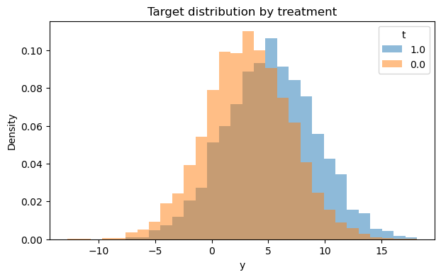
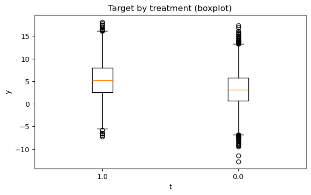
# 2) Outcome distribution by treatment (hist + boxplot)
fig1, fig2 = eda.outcome_plots()
plt.show()

Propensity

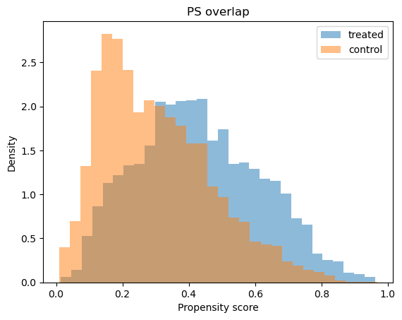
Now let’s examine how propensity score differ treatments

# Shows means of confounders for control/treated groups, absolute differences, and SMD values
confounders_balance_df = eda.confounders_means()
display(confounders_balance_df)

	mean_t_0	mean_t_1	abs_diff	smd
confounders
spend_last_month	90.313423	119.353025	29.039602	0.523162
premium_user	0.195066	0.354347	0.159281	0.362615
avg_sessions_week	4.902830	5.299702	0.396872	0.198761
urban_resident	0.576463	0.646805	0.070341	0.144688
tenure_months	23.329078	24.906290	1.577212	0.130648

# Propensity model fit
ps_model = eda.fit_propensity()

# ROC AUC - shows how predictable treatment is from confounders
roc_auc_score = ps_model.roc_auc
print("ROC AUC from PropensityModel:", round(roc_auc_score, 4))

ROC AUC from PropensityModel: 0.6937

# Positivity check - assess overlap between treatment groups
positivity_result = ps_model.positivity_check()
print("Positivity check from PropensityModel:", positivity_result)

Positivity check from PropensityModel: {'bounds': (0.05, 0.95), 'share_below': 0.0132, 'share_above': 0.0004, 'flag': False}

# SHAP values - feature importance for treatment assignment from confounders
shap_values_df = ps_model.shap
display(shap_values_df)

	feature	shap_mean
0	spend_last_month	-0.000735
1	tenure_months	0.000451
2	urban_resident	0.000190
3	premium_user	0.000124
4	avg_sessions_week	-0.000029

# Propensity score overlap graph
ps_model.ps_graph()
plt.show()

Outcome regression

Let’s analyze how confounders predict outcome

# Outcome model fit
outcome_model = eda.outcome_fit()

# RMSE and MAE of regression model
print(outcome_model.scores)

{'rmse': 3.6452253851701975, 'mae': 2.905800097741897}

# 2) SHAP values - feature importance for outcome prediction from confounders
shap_outcome_df = outcome_model.shap
display(shap_outcome_df)

	feature	shap_mean
0	premium_user	0.001378
1	avg_sessions_week	-0.001012
2	spend_last_month	-0.000987
3	urban_resident	0.000543
4	tenure_months	0.000078

Inference

Now time to estimate ATE with Double Machine Learning

from causalkit.inference.att import dml_att

# Estimate Average Treatment Effect (ATT)
att_result = dml_att(causal_data, n_folds=3, confidence_level=0.95)

att_result

{'coefficient': 1.3111886779440418,
 'std_error': 0.09481720872967514,
 'p_value': 1.7133685893213766e-43,
 'confidence_interval': (1.1253503637192617, 1.497026992168822),
 'model': <doubleml.irm.irm.DoubleMLIRM at 0x163ba74d0>}

Real ATT is 1.385

Refutation

# Import refutation utilities
from causalkit.refutation import (
    refute_placebo_outcome,
    refute_placebo_treatment,
    refute_subset,
    refute_irm_orthogonality,
    sensitivity_analysis,
    sensitivity_analysis_set
)

Placebo

Replacing outcome with dummy random variable must broke our model and effect will be near zero

# Replacing an outcome with placebo
att_placebo_outcome = refute_placebo_outcome(
    dml_att,
    causal_data,
    random_state=42
)

print(att_placebo_outcome)

{'theta': 0.0024891263554991036, 'p_value': 0.49268997429089034}

Replacing treatment with dummy random variable must broke our model and effect will be near zero

# Replacing treatment with placebo
att_placebo_treatment = refute_placebo_treatment(
    dml_att,
    causal_data,
    random_state=42
)

print(att_placebo_treatment)

{'theta': -0.004944799398107784, 'p_value': 0.9497270383821083}

Let’s chanllege our dataset and romove random parts. Theta shoul be near estimated

# Inference on subsets
subset_fractions = [0.3, 0.5]

att_subset_results = []
for fraction in subset_fractions:
    subset_result = refute_subset(
        dml_att,
        causal_data,
        fraction=fraction,
        random_state=42
    )
    att_subset_results.append(subset_result)

    print(f" With {fraction*100:.0f}% subset: theta = {subset_result['theta']:.4f}, p_value = {subset_result['p_value']:.4f}")

 With 30% subset: theta = 1.1546, p_value = 0.0000
 With 50% subset: theta = 1.3733, p_value = 0.0000

Orthogonality

Orthogonality tests validate whether our ATT estimator is properly specified. We will inspect:

• Out-of-sample (OOS) moment check;

• ATT-specific orthogonality derivatives (m0 and g only);

• Influence diagnostics;

• ATT overlap diagnostics and trim-sensitivity near m→1 (controls);

• Trimming info and overall diagnostic conditions.

att_ortho_check = refute_irm_orthogonality(dml_att, causal_data, target='ATT')

1. Out-of-sample moment check

print("\n--- 1. Out-of-Sample Moment Check ---")
oos_test = att_ortho_check['oos_moment_test']
print(f"T-statistic: {oos_test['tstat']:.4f}")
print(f"P-value: {oos_test['pvalue']:.4f}")
print(f"Interpretation: {oos_test['interpretation']}")
print("\nFold-wise results:")
display(oos_test['fold_results'])

--- 1. Out-of-Sample Moment Check ---
T-statistic: -0.2644
P-value: 0.7915
Interpretation: Should be ≈ 0 if moment condition holds

Fold-wise results:

	fold	n	psi_mean	psi_var
0	0	2000	0.329863	83.664056
1	1	2000	-0.573543	177.284891
2	2	2000	0.275107	89.104143
3	3	2000	0.177037	66.171971
4	4	2000	-0.339714	76.546856

psi_mean is expected to be near zero on every fold if the moment condition holds.

2. Orthogonality derivatives (ATT)

print("\n--- 2. Orthogonality (Gateaux Derivative) Tests — ATT ---")
ortho_derivs = att_ortho_check['orthogonality_derivatives']
print(f"Interpretation: {ortho_derivs['interpretation']}")

print("\nFull sample derivatives:")
display(ortho_derivs['full_sample'])

print("\nTrimmed sample derivatives:")
display(ortho_derivs['trimmed_sample'])

if len(ortho_derivs['problematic_full']) > 0:
    print("\n\u26A0 PROBLEMATIC derivatives (full sample):")
    display(ortho_derivs['problematic_full'])
else:
    print("\n\u2713 No problematic derivatives in full sample")

if len(ortho_derivs['problematic_trimmed']) > 0:
    print("\n\u26A0 PROBLEMATIC derivatives (trimmed sample):")
    display(ortho_derivs['problematic_trimmed'])
else:
    print("\n\u2713 No problematic derivatives in trimmed sample")

--- 2. Orthogonality (Gateaux Derivative) Tests — ATT ---
Interpretation: ATT: check m0 & g only; large |t| (>2) => calibration issues

Full sample derivatives:

	basis	d_m1	se_m1	t_m1	d_m0	se_m0	t_m0	d_g	se_g	t_g
0	0	0.0	0.0	0.0	0.029850	0.025167	1.186063	-1.009071	1.075327	-0.938385
1	1	0.0	0.0	0.0	0.011241	0.029021	0.387342	-2.351915	2.324239	-1.011908
2	2	0.0	0.0	0.0	0.005547	0.028698	0.193305	-1.938678	2.048945	-0.946184
3	3	0.0	0.0	0.0	0.022577	0.025612	0.881506	-1.069048	1.040382	-1.027554
4	4	0.0	0.0	0.0	0.000924	0.031841	0.029025	-2.086775	1.827563	-1.141835
5	5	0.0	0.0	0.0	-0.002677	0.024129	-0.110944	-0.829083	0.892210	-0.929247

Trimmed sample derivatives:

	basis	d_m1	se_m1	t_m1	d_m0	se_m0	t_m0	d_g	se_g	t_g
0	0	0.0	0.0	0.0	0.029844	0.025167	1.185838	-1.009999	1.075327	-0.939249
1	1	0.0	0.0	0.0	0.011255	0.029021	0.387832	-2.349584	2.324238	-1.010905
2	2	0.0	0.0	0.0	0.005538	0.028698	0.192966	-1.940275	2.048944	-0.946963
3	3	0.0	0.0	0.0	0.022581	0.025612	0.881691	-1.068271	1.040382	-1.026807
4	4	0.0	0.0	0.0	0.000927	0.031841	0.029127	-2.086239	1.827563	-1.141541
5	5	0.0	0.0	0.0	-0.002670	0.024129	-0.110656	-0.827944	0.892210	-0.927971

✓ No problematic derivatives in full sample

✓ No problematic derivatives in trimmed sample

For ATT, focus on t-statistics for m0 and g. Large absolute t-values (|t| > 2) suggest calibration issues.

3. Influence diagnostics

print("\n--- 3. Influence Diagnostics ---")
influence = att_ortho_check['influence_diagnostics']
print(f"Interpretation: {influence['interpretation']}")

print("\nFull sample influence metrics:")
print(f"  Plugin SE: {influence['full_sample']['se_plugin']:.4f}")
print(f"  Kurtosis: {influence['full_sample']['kurtosis']:.2f}")
print(f"  P99/Median ratio: {influence['full_sample']['p99_over_med']:.2f}")

print("\nTrimmed sample influence metrics:")
print(f"  Plugin SE: {influence['trimmed_sample']['se_plugin']:.4f}")
print(f"  Kurtosis: {influence['trimmed_sample']['kurtosis']:.2f}")
print(f"  P99/Median ratio: {influence['trimmed_sample']['p99_over_med']:.2f}")

print("\nTop influential observations (full sample):")
display(influence['full_sample']['top_influential'])

--- 3. Influence Diagnostics ---
Interpretation: Heavy tails or extreme kurtosis suggest instability

Full sample influence metrics:
  Plugin SE: 0.0993
  Kurtosis: 372.97
  P99/Median ratio: 8.23

Trimmed sample influence metrics:
  Plugin SE: 0.0993
  Kurtosis: 372.66
  P99/Median ratio: 8.20

Top influential observations (full sample):

	i	psi	g	res_t	res_c
0	5169	-433.731443	0.955891	0.0	6.953028
1	9369	-115.655411	0.768881	0.0	12.077354
2	5325	-92.729291	0.760111	0.0	10.166691
3	9615	-92.694582	0.829842	0.0	6.602995
4	4002	-80.529155	0.768305	0.0	8.436566
5	5990	77.598309	0.774365	-0.0	-7.854934
6	8342	-67.190692	0.776890	0.0	6.703443
7	313	-63.173514	0.777839	0.0	6.268191
8	7152	-61.702928	0.802739	0.0	5.267487
9	2958	-59.609550	0.721210	0.0	8.005001

4. ATT overlap diagnostics and trim-sensitivity

print("\n--- ATT Overlap Diagnostics ---")
overlap = att_ortho_check['overlap_diagnostics']
if overlap is not None:
    display(overlap)
else:
    print("Overlap diagnostics not available.")

print("\n--- ATT Trim-Sensitivity Curve ---")
robust = att_ortho_check['robustness']
trim_curve = robust.get('trim_curve', None) if robust is not None else None
if trim_curve is not None:
    display(trim_curve)
else:
    print("Trim-sensitivity curve not available.")

--- ATT Overlap Diagnostics ---

	threshold	pct_controls_with_g_ge_thr	pct_treated_with_g_le_1_minus_thr
0	0.95	0.015323	0.028785
1	0.97	0.000000	0.000000
2	0.98	0.000000	0.000000
3	0.99	0.000000	0.000000

--- ATT Trim-Sensitivity Curve ---

	trim_threshold	n	pct_dropped	theta	se
0	0.900000	9999	0.01	1.350662	0.090084
1	0.908636	9999	0.01	1.331246	0.091142
2	0.917273	9999	0.01	1.387317	0.092264
3	0.925909	9999	0.01	1.347702	0.090716
4	0.934545	9999	0.01	1.359888	0.091188
5	0.943182	9999	0.01	1.356327	0.090682
6	0.951818	9999	0.01	1.352705	0.091355
7	0.960455	10000	0.00	1.292609	0.096413
8	0.969091	10000	0.00	1.328536	0.094768
9	0.977727	10000	0.00	1.351585	0.092971
10	0.986364	10000	0.00	1.346071	0.095060
11	0.995000	10000	0.00	1.359726	0.092266

5. Propensity score trimming

print("\n--- Propensity Score Trimming ---")
trim_info = att_ortho_check['trimming_info']
print(f"Trimming bounds: {trim_info['bounds']}")
print(f"Observations trimmed: {trim_info['n_trimmed']} ({trim_info['pct_trimmed']:.1f}%)")

--- Propensity Score Trimming ---
Trimming bounds: (0.02, 0.98)
Observations trimmed: 1 (0.0%)

6. Diagnostic conditions breakdown

print("\n--- Diagnostic Conditions Assessment ---")
conditions = att_ortho_check['diagnostic_conditions']
print("Individual condition checks:")
for condition, passed in conditions.items():
    status = "\u2713 PASS" if passed else "\u2717 FAIL"
    print(f"  {condition}: {status}")

print(f"\nOverall: {att_ortho_check['overall_assessment']}")

--- Diagnostic Conditions Assessment ---
Individual condition checks:
  oos_moment_ok: ✓ PASS
  derivs_full_ok: ✓ PASS
  derivs_trim_ok: ✓ PASS
  se_reasonable: ✓ PASS
  no_extreme_influence: ✓ PASS
  trimming_reasonable: ✓ PASS

Overall: PASS: Strong evidence for orthogonality

Sensitivity analysis

Let’s analyze how unobserved confounder could look

bench_sets = causal_data.confounders
res = sensitivity_analysis_set(
    att_result,
    benchmarking_set=bench_sets,
    level=0.95,
    null_hypothesis=0.0,
)

# Build a DataFrame with confounders as rows and the metrics as columns
summary_df = pd.DataFrame({
    name: (df.loc['t'] if 't' in df.index else df.iloc[0])
    for name, df in res.items()
}).T

summary_df

	cf_y	cf_d	rho	delta_theta
tenure_months	0.052112	0.004799	0.534682	0.069932
avg_sessions_week	0.033761	0.017667	0.828866	0.166359
spend_last_month	0.023657	0.081000	1.000000	0.385810
premium_user	0.039786	0.047103	0.646352	0.226695
urban_resident	0.000000	0.011797	1.000000	0.023253

It is business domain and data knowledge relative question. In this situation we will stop on the most influential confounder ‘spend_last_month’ and test theta when we do not observe another confounder with strength of ‘premium_user’

# Run sensitivity analysis on our ATT result
sensitivity_report_1 = sensitivity_analysis(
    att_result,
    cf_y=0.02,  # Confounding strength affecting outcome
    cf_d=0.08,  # Confounding strength affecting treatment
    rho=1.0     # Perfect correlation between unobserved confounders
)

print(sensitivity_report_1)

================== Sensitivity Analysis ==================

------------------ Scenario          ------------------
Significance Level: level=0.95
Sensitivity parameters: cf_y=0.02; cf_d=0.08, rho=1.0

------------------ Bounds with CI    ------------------
   CI lower  theta lower     theta  theta upper  CI upper
t  0.804583     0.965456  1.311189     1.656921  1.809618

------------------ Robustness Values ------------------
   H_0     RV (%)    RVa (%)
t  0.0  14.614512  12.772404

CI lower >> 0. It means test is passed