DML ATE Example

This notebook covers scenario:

Is RCT	Treatment	Outcome	EDA	Estimands	Refutation
Observational	Binary	Continuous	Yes	ATE	Yes

We will estimate Average Treatment Effect (ATE) of binary treatment on continuous outcome. It shows explonatary data analysis and refutation tests

Generate data

Let’s generate data of how feature (Treatment) impact on ARPU (Outcome) with linear effect (theta) = 1.8

import numpy as np
import pandas as pd
import matplotlib.pyplot as plt
from causalis.data import CausalDatasetGenerator, CausalData

# Reproducibility
np.random.seed(42)

confounder_specs = [
    {"name": "tenure_months", "dist": "normal", "mu": 24, "sd": 12},
    {"name": "avg_sessions_week", "dist": "normal", "mu": 5, "sd": 2},
    {"name": "spend_last_month", "dist": "uniform", "a": 0, "b": 200},
    {"name": "premium_user", "dist": "bernoulli", "p": 0.25},
    {"name": "urban_resident", "dist": "bernoulli", "p": 0.60},
]

# Causal effect and noise
theta = 1.8  # ATE: +1.8 ARPU units if new_feature = 1
sigma_y = 3.5  # ARPU noise std
target_d_rate = 0.2  # ~20% treated

# Effects of confounders on ARPU (baseline, additive)
# Order: tenure_months, avg_sessions_week, spend_last_month, premium_user, urban_resident
beta_y = np.array([
    0.05,  # tenure_months: small positive effect
    0.40,  # avg_sessions_week: strong positive effect
    0.02,  # spend_last_month: recent spend correlates with ARPU
    2.00,  # premium_user: premium users have higher ARPU
    1.00,  # urban_resident: urban users slightly higher ARPU
], dtype=float)

# Effects of confounders on treatment assignment (log-odds scale)
beta_d = np.array([
    0.015,  # tenure_months
    0.10,  # avg_sessions_week
    0.002,  # spend_last_month
    0.75,  # premium_user
    0.30,  # urban_resident: more likely to get the feature
], dtype=float)

gen = CausalDatasetGenerator(
    theta=theta,
    outcome_type="continuous",
    sigma_y=sigma_y,
    target_d_rate=target_d_rate,
    seed=42,
    confounder_specs=confounder_specs,
    beta_y=beta_y,
    beta_d=beta_d,
)


# Create dataset
causal_data = gen.to_causal_data(
    n=10_000,
    confounders = [
    "tenure_months",
    "avg_sessions_week",
    "spend_last_month",
    "premium_user",
    "urban_resident",
]
)

# Show first few rows
causal_data.df.head()

	y	d	tenure_months	avg_sessions_week	spend_last_month	premium_user	urban_resident
0	4.127714	0.0	27.656605	5.352554	72.552568	1.0	0.0
1	11.122008	1.0	11.520191	6.798247	188.481287	1.0	0.0
2	10.580393	1.0	33.005414	2.055459	51.040440	0.0	1.0
3	6.982844	1.0	35.286777	4.429404	166.992239	0.0	1.0
4	10.899381	0.0	0.587578	6.658307	179.371126	0.0	0.0

EDA

from causalis.eda import CausalEDA
eda = CausalEDA(causal_data)

# shape of data
eda.data_shape()

{'n_rows': 10000, 'n_columns': 7}

General dataset information

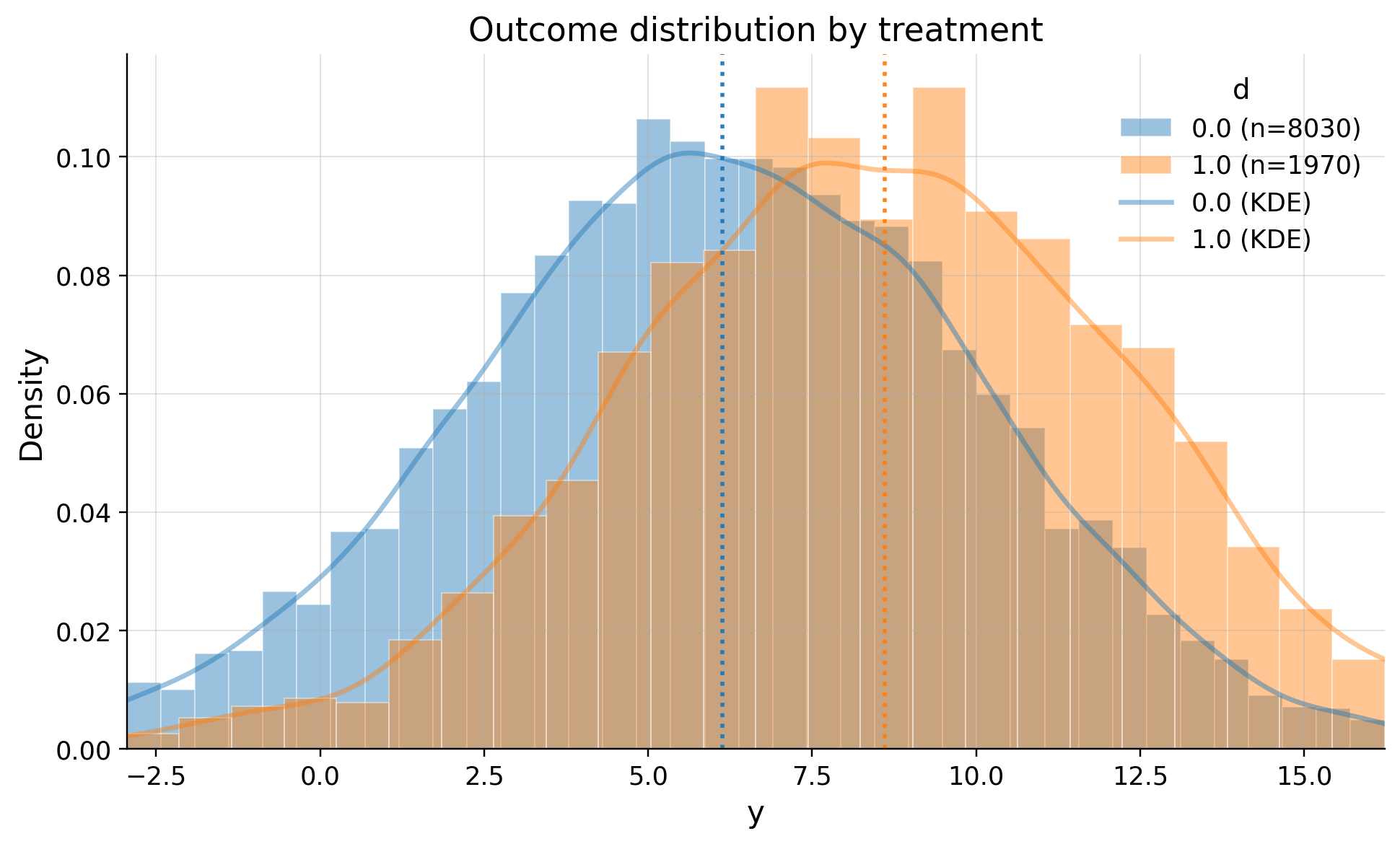
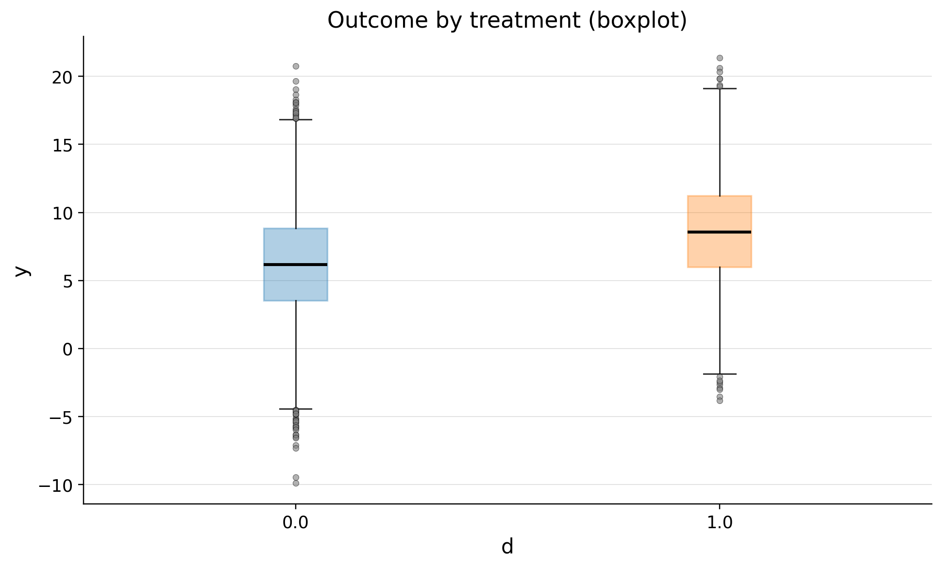
Let’s see how outcome differ between clients who recieved the feature and didn’t

# 1) Outcome statistics by treatment
eda.outcome_stats()

	count	mean	std	min	p10	p25	median	p75	p90	max
treatment
0.0	8030	6.137433	3.933863	-9.866447	1.118291	3.517427	6.157583	8.847907	11.114776	20.770359
1.0	1970	8.608973	3.942856	-3.821492	3.666892	5.986613	8.560912	11.247429	13.552612	21.377687

eda.outcome_hist()

eda.outcome_boxplot()

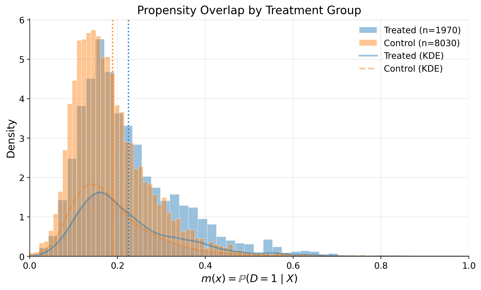
Propensity

Now let’s examine how propensity score differ treatments

# Shows means of confounders for control/treated groups, absolute differences, and SMD values
confounders_balance_df = eda.confounders_means()
display(confounders_balance_df)

	mean_t_0	mean_t_1	abs_diff	smd	ks	ks_pvalue
confounders
premium_user	0.218057	0.382234	0.164176	0.364037	0.164176	1.061599e-37
tenure_months	23.405355	25.799499	2.394143	0.199024	0.087485	5.511096e-11
avg_sessions_week	4.976354	5.302999	0.326645	0.163509	0.075782	2.382131e-08
urban_resident	0.587547	0.655330	0.067783	0.140072	0.067783	9.127269e-07
spend_last_month	99.288113	104.941250	5.653137	0.097172	0.057348	5.761025e-05

# Propensity model fit
ps_model = eda.fit_propensity()

# ROC AUC - shows how predictable treatment is from confounders
roc_auc_score = ps_model.roc_auc
print("ROC AUC from PropensityModel:", round(roc_auc_score, 4))

ROC AUC from PropensityModel: 0.5926

# Positivity check - assess overlap between treatment groups
positivity_result = ps_model.positivity_check()
print("Positivity check from PropensityModel:", positivity_result)

Positivity check from PropensityModel: {'bounds': (0.05, 0.95), 'share_below': 0.0121, 'share_above': 0.0, 'flag': False}

# SHAP values - feature importance for treatment assignment from confounders
shap_values_df = ps_model.shap
display(shap_values_df)

	feature	shap_mean	shap_mean_abs	exact_pp_change_abs	exact_pp_change_signed
0	num__spend_last_month	0.000299	0.166002	0.027438	0.000047
1	num__premium_user	-0.000269	0.306301	0.052687	-0.000042
2	num__urban_resident	0.000245	0.158900	0.026210	0.000039
3	num__avg_sessions_week	-0.000141	0.174082	0.028841	-0.000022
4	num__tenure_months	-0.000135	0.194878	0.032482	-0.000021

# Propensity score overlap graph
ps_model.plot_m_overlap()

Outcome regression

Let’s analyze how confounders predict outcome

# Outcome model fit
outcome_model = eda.outcome_fit()

# RMSE and MAE of regression model
print(outcome_model.scores)

{'rmse': 3.656989617205263, 'mae': 2.90424413216463}

# 2) SHAP values - feature importance for outcome prediction from confounders
shap_outcome_df = outcome_model.shap
display(shap_outcome_df)

	feature	shap_mean
0	avg_sessions_week	-0.000502
1	spend_last_month	0.000350
2	urban_resident	0.000245
3	premium_user	-0.000055
4	tenure_months	-0.000038

Inference

Now time to estimate ATE with Double Machine Learning

from causalis.inference.ate import dml_ate

# Estimate Average Treatment Effect (ATE)
ate_result = dml_ate(causal_data, n_folds=4, confidence_level=0.95)

print(ate_result.get('coefficient'))
print(ate_result.get('p_value'))
print(ate_result.get('confidence_interval'))

1.766253520771568
0.0
(1.5329683790491713, 1.9995386624939646)

True theta in our data generating proccess was 1.8

Refutation

Overlap

from  causalis.refutation import *
rep = run_overlap_diagnostics(res=ate_result)
rep["summary"]

	metric	value	flag
0	edge_0.01_below	0.000000	GREEN
1	edge_0.01_above	0.000000	GREEN
2	edge_0.02_below	0.001000	GREEN
3	edge_0.02_above	0.000000	GREEN
4	KS	0.139672	GREEN
5	AUC	0.592382	GREEN
6	ESS_treated_ratio	0.742224	GREEN
7	ESS_control_ratio	0.970455	GREEN
8	tails_w1_q99/med	6.278831	GREEN
9	tails_w0_q99/med	2.844508	GREEN
10	ATT_identity_relerr	0.037683	GREEN
11	clip_m_total	0.000100	GREEN
12	calib_ECE	0.036215	GREEN
13	calib_slope	0.520588	RED
14	calib_intercept	-0.637457	RED

Score

from causalis.refutation.score.score_validation import run_score_diagnostics
rep_score = run_score_diagnostics(res=ate_result)
rep_score["summary"]

	metric	value	flag
0	se_plugin	1.190252e-01	NA
1	psi_p99_over_med	1.355647e+01	YELLOW
2	psi_kurtosis	6.047594e+01	RED
3	max_|t|_g1	5.463687e+00	RED
4	max_|t|_g0	1.384511e+00	GREEN
5	max_|t|_m	1.388284e+00	GREEN
6	oos_tstat_fold	1.241609e-15	GREEN
7	oos_tstat_strict	1.241615e-15	GREEN

SUTVA

print_sutva_questions()

1.) Are your clients independent (i)?
2.) Do you measure confounders, treatment, and outcome in the same intervals?
3.) Do you measure confounders before treatment and outcome after?
4.) Do you have a consistent label of treatment, such as if a person does not receive a treatment, he has a label 0?

Uncofoundedness

from causalis.refutation.unconfoundedness.uncofoundedness_validation import run_unconfoundedness_diagnostics

rep_uc = run_unconfoundedness_diagnostics(res=ate_result)
rep_uc['summary']

	metric	value	flag
0	balance_max_smd	0.021956	GREEN
1	balance_frac_violations	0.000000	GREEN

from causalis.refutation.unconfoundedness.sensitivity import (
    sensitivity_analysis, sensitivity_benchmark
)

sensitivity_analysis(ate_result, cf_y=0.01, cf_d=0.01, rho=1.0, level=0.95)

{'theta': 1.766253520771568,
 'se': 0.11902521860734187,
 'level': 0.95,
 'z': 1.959963984540054,
 'sampling_ci': (1.5329683790491713, 1.9995386624939646),
 'theta_bounds_confounding': (1.6875916811818483, 1.8449153603612876),
 'bias_aware_ci': (1.4543065394594517, 2.0782005020836842),
 'max_bias': 0.07866183958971962,
 'sigma2': 13.136641553423134,
 'nu2': 0.43676740621591587,
 'params': {'cf_y': 0.01, 'cf_d': 0.01, 'rho': 1.0, 'use_signed_rr': False}}

sensitivity_benchmark(ate_result, benchmarking_set =['tenure_months'])

	cf_y	cf_d	rho	theta_long	theta_short	delta
d	0.000034	3.037675e-07	-1.0	1.766254	1.845679	-0.079425