DML GATE Example#
This notebook demonstrates how to estimate Group Average Treatment Effects (GATE) using Double Machine Learning. GATE allows us to understand treatment effect heterogeneity by estimating the average effect within specific groups defined by covariates.
Mathematical Formulation#
Let \(Y\) be the outcome, \(D\) the binary treatment, and \(X\) the covariates. We define the Conditional Average Treatment Effect (CATE) as:
For a set of groups \(G_1, \dots, G_K\) (where \(G_k(X)\) is an indicator that unit falls into group \(k\)), the GATE for group \(k\) is:
We will:
Generate synthetic data with heterogeneous treatment effects.
Perform Exploratory Data Analysis (EDA).
Estimate GATEs using
gate_esimandwith both automatic quantile groups and custom user-defined groups.
Generate data#
We generate observational data with a nonlinear outcome model, nonlinear treatment assignment, and a heterogeneous (nonlinear) treatment effect \(\tau(X)\).
import numpy as np
import pandas as pd
import matplotlib.pyplot as plt
from causalis.data import CausalDatasetGenerator, CausalData

# Reproducibility
np.random.seed(42)

# 1) Confounders and their distributions
confounder_specs = [
    {"name": "tenure_months",     "dist": "normal",   "mu": 24, "sd": 12},
    {"name": "avg_sessions_week", "dist": "normal",   "mu": 5,  "sd": 2},
    {"name": "spend_last_month",  "dist": "uniform",  "a": 0,   "b": 200},
    {"name": "premium_user",      "dist": "bernoulli","p": 0.25},
    {"name": "urban_resident",    "dist": "bernoulli","p": 0.60},
]

# Indices
TENURE, SESS, SPEND, PREMIUM, URBAN = range(5)

# 2) Nonlinear baseline for outcome f_y(X) = X @ beta_y + g_y(X)
beta_y = np.array([0.03, 0.20, 0.01, 1.20, 0.60], dtype=float)

def g_y(X: np.ndarray) -> np.ndarray:
    tenure_years = X[:, TENURE] / 12.0
    sessions = X[:, SESS]
    spend = X[:, SPEND]
    premium = X[:, PREMIUM]
    urban = X[:, URBAN]
    return (
        1.2 * np.sin(2.0 * np.pi * tenure_years)
        + 0.02 * (sessions - 5.0) ** 2
        + 0.0015 * (spend - 100.0) * (sessions - 5.0)
        + 0.4 * premium * (sessions - 5.0)
        + 0.3 * urban * np.tanh((spend - 100.0) / 50.0)
    )

# 3) Nonlinear treatment score f_t(X) = X @ beta_t + g_t(X)
beta_d = np.array([0.010, 0.12, 0.001, 0.80, 0.25], dtype=float)

def g_d(X: np.ndarray) -> np.ndarray:
    tenure_years = X[:, TENURE] / 12.0
    sessions = X[:, SESS]
    spend = X[:, SPEND]
    premium = X[:, PREMIUM]
    urban = X[:, URBAN]
    soft_spend = 1.2 * np.tanh((spend - 80.0) / 40.0)
    return (
        0.6 * soft_spend
        + 0.15 * (sessions - 5.0) * (tenure_years - 2.0)
        + 0.25 * premium * (urban - 0.5)
    )

# 4) Heterogeneous, nonlinear treatment effect tau(X)
def tau_fn(X: np.ndarray) -> np.ndarray:
    tenure_years = X[:, TENURE] / 12.0
    sessions = X[:, SESS]
    spend = X[:, SPEND]
    premium = X[:, PREMIUM]
    urban = X[:, URBAN]
    tau = (
        1.0
        + 0.8 * (1.0 / (1.0 + np.exp(-(sessions - 5.0))))
        + 0.5 * premium
        - 0.6 * np.clip(tenure_years / 5.0, 0.0, 1.0)
        + 0.2 * urban * (spend - 100.0) / 100.0
    )
    return np.clip(tau, 0.2, 2.5)

# 5) Noise and prevalence
sigma_y = 3.5
target_d_rate = 0.35

# 6) Build generator
gen = CausalDatasetGenerator(
    outcome_type="continuous",
    sigma_y=sigma_y,
    target_d_rate=target_d_rate,
    seed=42,
    confounder_specs=confounder_specs,
    beta_y=beta_y,
    beta_d=beta_d,
    g_y=g_y,
    g_d=g_d,
    tau=tau_fn,
)

# 7) Generate data
n = 10000
generated_df = gen.generate(n)

# Ground-truth ATT
true_att = float(generated_df.loc[generated_df["d"] == 1, "cate"].mean())
print(f"Ground-truth ATT from the DGP: {true_att:.3f}")

# 8) Wrap as CausalData
causal_data = CausalData(
    df=generated_df,
    treatment="d",
    outcome="y",
    confounders=[
        "tenure_months",
        "avg_sessions_week",
        "spend_last_month",
        "premium_user",
        "urban_resident",
    ],
)

causal_data.df.head()
Ground-truth ATT from the DGP: 1.386
| y | d | tenure_months | avg_sessions_week | spend_last_month | premium_user | urban_resident | |
|---|---|---|---|---|---|---|---|
| 0 | 2.237316 | 0.0 | 27.656605 | 5.352554 | 72.552568 | 1.0 | 0.0 |
| 1 | 5.771469 | 0.0 | 11.520191 | 6.798247 | 188.481287 | 1.0 | 0.0 |
| 2 | 6.374653 | 1.0 | 33.005414 | 2.055459 | 51.040440 | 0.0 | 1.0 |
| 3 | 2.364177 | 1.0 | 35.286777 | 4.429404 | 166.992239 | 0.0 | 1.0 |
| 4 | 8.378079 | 0.0 | 0.587578 | 6.658307 | 179.371126 | 0.0 | 0.0 |
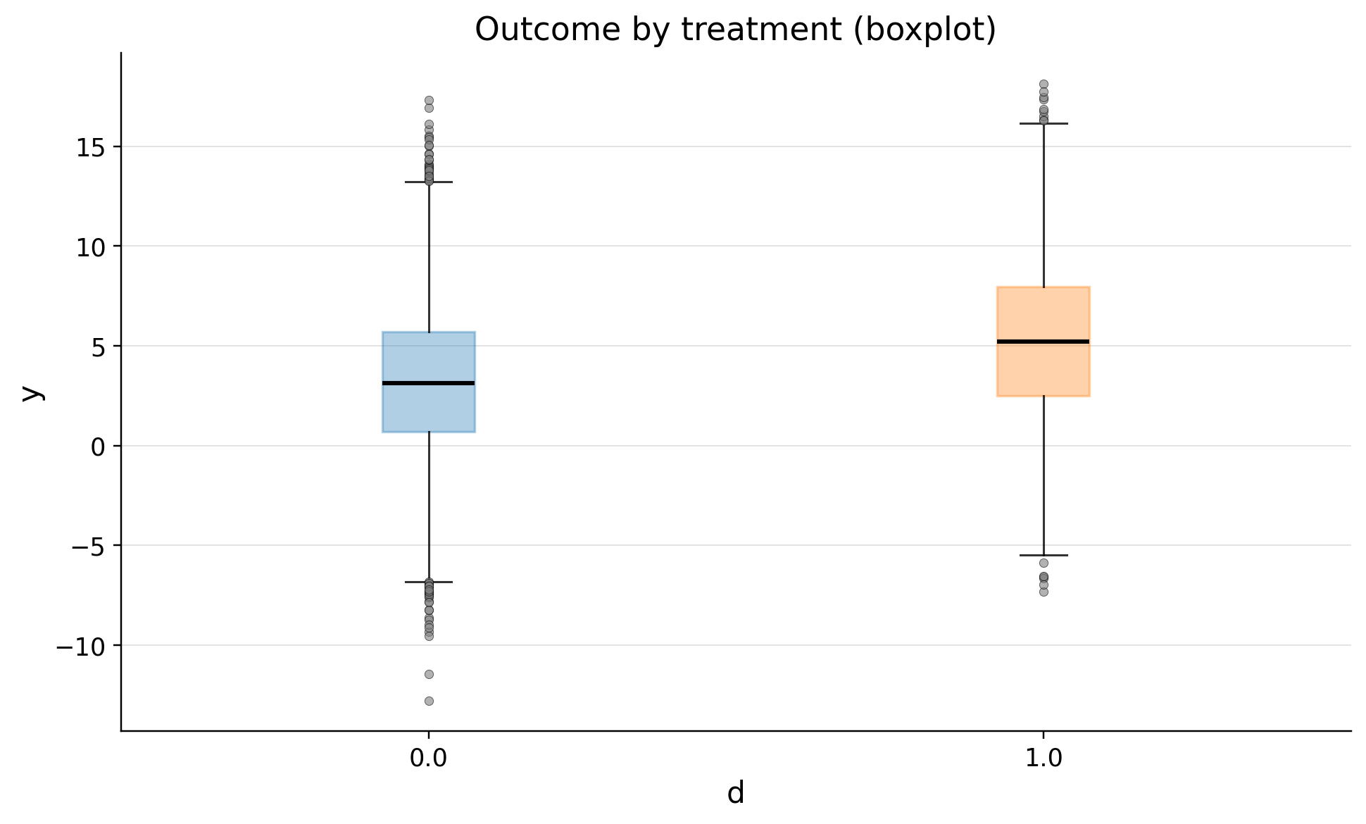
EDA#
from causalis.eda import CausalEDA
eda = CausalEDA(causal_data)
eda.outcome_stats()
eda.outcome_hist()
eda.outcome_boxplot()
Inference: Estimating GATE#
We use gate_esimand to estimate Group Average Treatment Effects.
This function works by leveraging the orthogonal signal from the DoubleML framework.
Methodology#
Orthogonal Signal: We fit a DoubleML IRM model to obtain a score \(\psi(W;\hat{\eta})\) such that:
\[ \mathbb{E}[\psi(W; \hat{\eta}) \mid X] \approx \tau(X) \]where \(W = (Y, D, X)\) and \(\hat{\eta}\) are the estimated nuisance parameters.
Best Linear Predictor (BLP): We assume a linear model for the CATE using group indicators \(G(X)\):
\[ \tau(X) \approx \sum_k \theta_k G_k(X) \]We estimate coefficients \(\theta\) by solving the BLP optimization:
\[ \hat{\theta} = \arg\min_{\theta} \sum_{i=1}^N (\psi(W_i) - \theta^\top G(X_i))^2\]
When \(G(X)\) consists of mutually exclusive group indicators, \(\hat{\theta}_k\) corresponds to the average of the orthogonal signal within group \(k\), providing a consistent estimate of the GATE.
from causalis.inference.gate.gate_esimand import gate_esimand
1. GATE by CATE Quantiles#
If no groups are provided, gate_esimand automatically creates groups based on quantiles of the estimated CATE (Conditional Average Treatment Effect).
# Estimate GATE with 5 quantile groups
gate_quantiles = gate_esimand(causal_data, n_groups=5, confidence_level=0.95)

print("GATE Results (Quantiles):")
display(gate_quantiles)
GATE Results (Quantiles):
| group | n | theta | std_error | p_value | ci_lower | ci_upper | |
|---|---|---|---|---|---|---|---|
| 0 | Group_0 | 2000 | 1.376851 | 0.212620 | 9.441200e-11 | 0.960123 | 1.793579 |
| 1 | Group_1 | 2000 | 0.899152 | 0.196052 | 4.512072e-06 | 0.514896 | 1.283408 |
| 2 | Group_2 | 2000 | 1.114911 | 0.194088 | 9.226342e-09 | 0.734507 | 1.495316 |
| 3 | Group_3 | 2000 | 1.190621 | 0.188706 | 2.801072e-10 | 0.820765 | 1.560478 |
| 4 | Group_4 | 2000 | 1.332698 | 0.207103 | 1.235086e-10 | 0.926784 | 1.738612 |
2. GATE by User-Defined Groups#
We can also define custom groups based on covariates. For example, let’s group users by their tenure:
< 1 year
1-3 years
> 3 years
# Define custom groups
tenure = causal_data.df['tenure_months']
groups = pd.cut(tenure, bins=[-np.inf, 12, 36, np.inf], labels=['<1y', '1-3y', '>3y'])

# Estimate GATE
gate_custom = gate_esimand(causal_data, groups=groups, confidence_level=0.95)

print("GATE Results (Tenure Groups):")
display(gate_custom)
GATE Results (Tenure Groups):
| group | n | theta | std_error | p_value | ci_lower | ci_upper | |
|---|---|---|---|---|---|---|---|
| 0 | tenure_months_1-3y | 6785 | 1.187370 | 0.107453 | 2.189553e-28 | 0.976765 | 1.397974 |
| 1 | tenure_months_<1y | 1649 | 1.231591 | 0.221586 | 2.727795e-08 | 0.797290 | 1.665891 |
| 2 | tenure_months_>3y | 1566 | 1.104541 | 0.221472 | 6.123645e-07 | 0.670464 | 1.538617 |
# Plot the results
plt.figure(figsize=(10, 6))

# Calculate error bars (distance from the mean)
yerr = [
    gate_custom['theta'] - gate_custom['ci_lower'],
    gate_custom['ci_upper'] - gate_custom['theta']
]

plt.errorbar(
    x=gate_custom['group'].astype(str),
    y=gate_custom['theta'],
    yerr=yerr,
    fmt='o',
    capsize=5,
    label='GATE Estimate'
)

plt.axhline(0, color='gray', linestyle='--', alpha=0.7)
plt.xlabel('Group')
plt.ylabel('GATE')
plt.title('Group Average Treatment Effects (Custom Groups)')
plt.legend()
plt.grid(axis='y', alpha=0.3)
plt.show()